Real 3-d climate is often analysed under the assumption that the climate state is constant and the weather is a deviation from this climate state. This means a point climate or climate dimension 0 in phase space. A more advanced analysis would assume that the climate state is not a point in phase space but rather a state depending on parameters c1, ..., cn, where n is a small number. From the argument given above it follows that n must be small in order to analyse it using just a few available measurements. Very little work has been done beyond the point climate model for the real atmosphere.
However for simplified climate systems this is more easy to analyse and the Lorenz model is an example often used to imagine howw the real climate may look like. In particular the Lorenz model shows climate bifurcation, which should be a point of concern, if in the real climate it would occur also. In this place we try to give a system of looking at the Lorenz climate bifurcation without a detailed mathematical understanding and no programming skills in Unix and Fortran and still alto do climate runs of his / her own.
While sometimes the Lorenz model is presented as a purely algebraic construction, we here want to emphasize that it describes real atmospheric flow for a simplified geometry. The Lorenz model describes the circulation in a rectangular cave, which is heated from below and cooled above. The circulation depends on parameters which describe the flow, such as length, height and viscosity of the air. Commonly these are given by non-dimensional parameters. For our rectangular cave these are: Reynolds number Re, describing the viscosity of the air, the Rayley number Ra being connected to the temperature difference between top and bottom and the Prantl number Pr conncted to the surface friction. Note that the physical situation and the flow inside the area are the same whenever these three numbers are the same. This means that caves of the different size may have the same flow solution when the non-dimensional parameters are equal.
The theory is described in [1] and [2]. The systems have been experimentally realized and simulated by high dimensional numerical models and for some values of Re,Ra, Pr the low dimensional Lorenz model simulates the flow well. When using the same terminology as with the real climate system on the sphere, we call the high dimensional model a general circulation model and the Lorenz model the climate dynamics model.
The reader with an interest in this theory and some (small) programming skills can obtain a account on our server and do some Lorenz experiments on his/her own. In particular the dependence of the the climate bifurcation on Re,Ra,Pr can be explored using the software provided.
In this WEB application we want to give the opportunity to experiment with initial values of the Lorenz models with only rudimentary mathematical skills and no knowledge of Unix/Linux and Fortran. The phase space the Lorenz model is three dimensional and the amplitudes are called A, T1 and T2. These amplitudes are time dependent describing the climate development in time. For A,T1 and T2 initial values must be provided and the time development is computed in time steps of dt, where here a default value of dt=.1 is used.
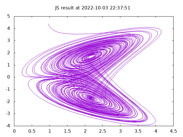
The initial values can be chosen from the whole 3 dimensional space. However, the solution curves do not cover the whole 3-d area, but rather fill two two dimensional surfaces, which are connected and the solution curve changes between these surface. While at first sight the cuves in each sheet seem to obe periodic, they are not and never come back to the same value. They are also chaotic, meaning unpredictable. After some prediction time the two solutions differ by a large amount, when at the start time the solutions have only a tiny difference. There is a predictive time of total chaos. This means that when the difference of two initial values goes to 0, the curves obtain a maximum difference.
In the fig. 1 above the initial value was chosen inside the attractor. Any value can be chosen and the solution the goes rather fast towards the attractor. The simple Lorenz model can be used to experiment with different initial values, estimate the predictice time and the chaotic regime and more.